

Welcome to this step-by-step guide to create time-to animations in QGIS.
Update: IE users, you’ll have to download the videos as webm videos are not supported by your browser. If you want to see the videos onsite, change to another browser like Firefox or Chrome
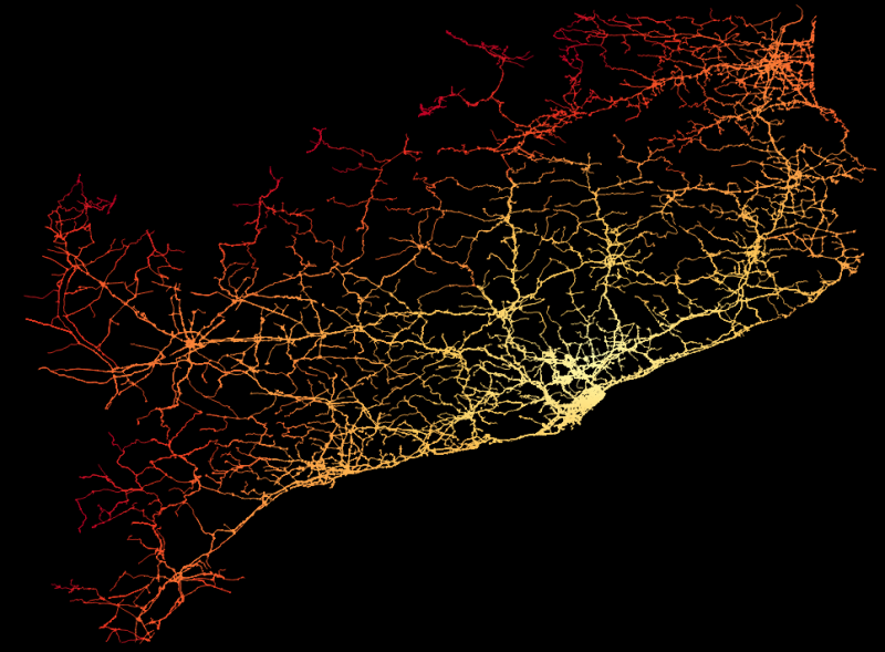
Here is an example of what we’ll do in this article:
Step 1: Installing the needed software
First of all, a list of what we are going to need:
- PostgreSQL
- PostGIS
- pgRouting
- OSM data
- QGIS
- TimeManager plugin
- ffmpeg
If you have everything you can skip to step 2.
Follow this steps:
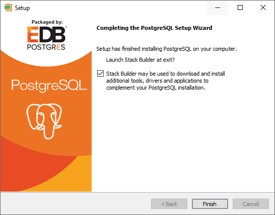
- Download PostgreSQL 9.6 from EnterpriseDB
- After installing you will be prompted to launch Stack Builder. Check the option and press finish.
- Select your installation, proceed and select PostGIS 2.4 Bundle for PostgreSQL 9.6 under Spatial Extensions
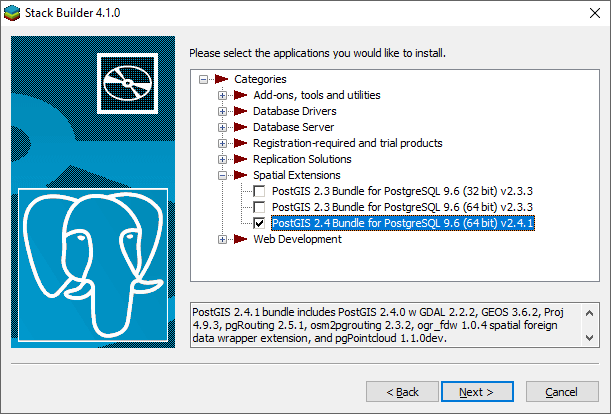
- The PostGIS installation will autodetect your PostgreSQL installation and configure itself. During the installation you will be prompted to enable different settings (Raster drivers and raster out of db). Those are used to enable PostGIS to raster output. We will not be using that but you might want to enable them to use them in the future.
- If you have followed the instructions and installed PostGIS from the PostGIS bundle, pgRouting will already be installed. If you don’t, you can install it from here
- Download pgAdmin from here and configure it to connect to our new PostgreSQL server.
- Go to Object -> Create Server
- Enter a name
- Set Connection to 127.0.0.1
- Set the Username and Password fields to the ones you set when installing PostgreSQL and press Ok
- You’ll see the server on the left hand panel. Open it and right click on Databases -> Create -> Database. We’ll name the database routing
- Install QGIS from here. I’ve been using QGIS 2.18.13 but anything newer should work.
- Open QGIS and install the TimeManager plugin:
- Go to Plugins -> Manage and Install plugins
- Search for TimeManager using the search box and install it. After installing you will see that a new panel is displayed below the main area
- Download and install ffmpeg from this link
Now that everything is installed we should download search some data to work with
Step 2: Download OSM data
We have two options to download OSM data: Using one of mapzen’s metro extracts or downloading a custom area using the OSM Overpass API
Using mapzen’s metro extracts:
Select one of the regions you are interested in and download the XML Raw OpenStreetMap dataset. The data will be downloaded in a bz2 file. You can use 7zip to extract it.
Although this is the easiest way to download data, the downloaded data includes a lot of data we won’t be using.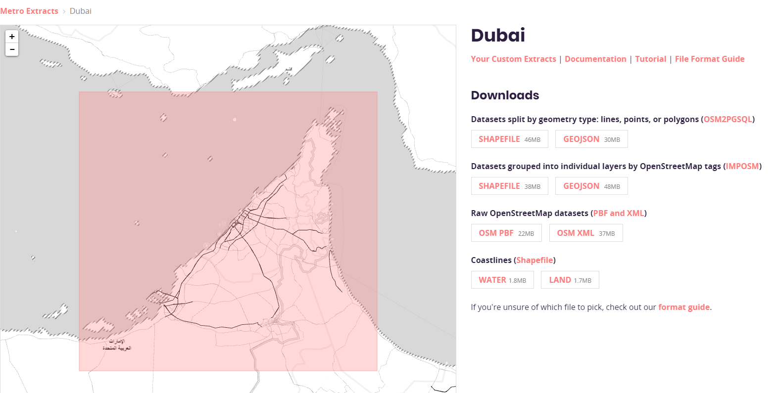
Downloading a custom area:
If you want to use a custom area or you don’t want anything to do with the hassle of downloading data you won’t need, we can use the Overpass API to download it.
Overpass has its own powerful query language to download data from a bounding box, unfortunately we can’t see which data we are downloading before we open it. Fortunately for us Overpass Turbo provides a graphical interface to see the data we are downloading so we can refine our search.
Overpass Turbo has two panels. A left one where the search query is written and another one that defines the bounding box through a map view.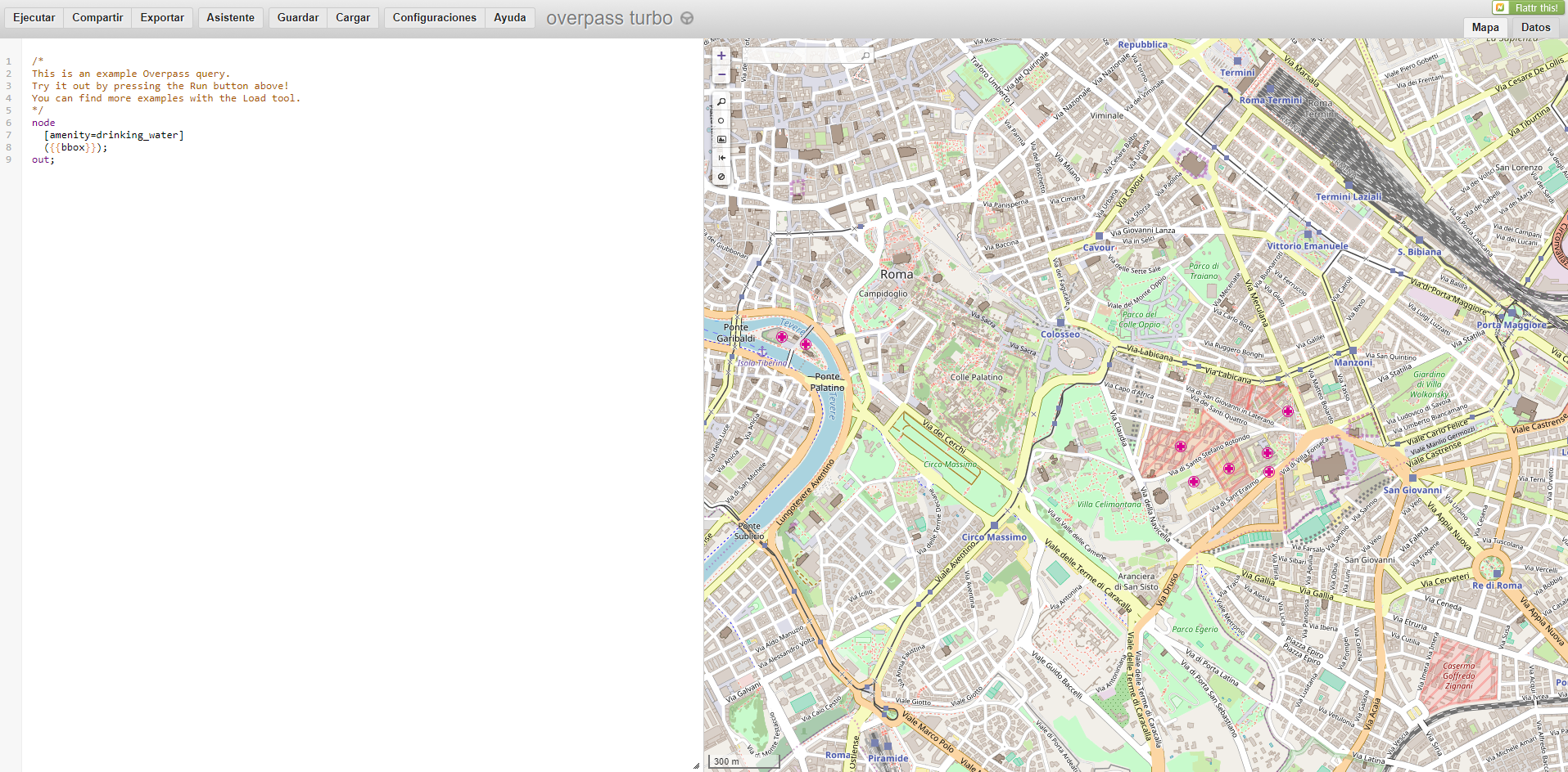
Enter the following query in the left panel:
[bbox:{{bbox}}];
way[highway~"^(motorway|motorway_link|motorway_junction|trunk|trunk_link|trunk_junction|primary|primary_link|primary_junction|secondary|secondary_link|secondary_junction|tertiary|tertiary_link|tertiary_junction)$"];
>;
out meta;
way[highway~"^(motorway|motorway_link|motorway_junction|trunk|trunk_link|trunk_junction|primary|primary_link|primary_junction|secondary|secondary_link|secondary_junction|tertiary|tertiary_link|tertiary_junction)$"];
out meta;
Line 1 selects the current bounding box as the search area
Line 2 selects the enclosed way elements using the highway key and searches for all the motorways, trunks, primary, secondary and tertiary roads and their junks and links. You can see a full list of attribute values here.
Line 3 looks for the child nodes of the previous set
Line 4 prints all their data
Line 5 selects all the ways inside the bounding box again
Line 6 prints all their data
Some considerations about the query:
- If you want to get city streets you should add residential to the highway type list
- If you look closely you’ll see that we are repeating the way search twice. While inserting the data to the database we’ll use a tool called osm2pgrouting that needs the nodes to be defined before the ways they are used in are.
That’s why we are getting the ways, looking for all their descendant nodes with the > operator and printing them. Then we need to print the ways so we look for them again.
Notice that we can’t use the parent operator (<) as that will include nodes not referenced in the file (the ones outside the bounding box).
Press Run to run the query. A warning might appear if a lot of data is going to be downloaded. After it finishes we should see the selected data in the map panel.
Press the export button and select Raw data. That will generate an OSM XML formatted file that can be used by osm2pgrouting.
Step 3: Inserting the data into postgreSQL
To use osm2pgrouting we need a mapconfig.xml file that filters out the data found in the OSM XML file. I’m using the one found here as that keeps the data we are interested in. Download it and put it in the same folder where you have downloaded the OSM data.
We are going to use a tool named osm2pgrouting that comes with pgrouting and does exactly what we want: Imports OSM data into PostgreSQL.
Open a command line tool and go to the PostgreSQL bin directory (in Windows that’s located in C:\Program Files\PostgreSQL\9.6\bin) and run the following command (change your paths, the database name, the username and password accordingly):
./osm2pgrouting.exe --f /path/to/osmFile.osm --conf /path/to/mapconfig.xml --dbname routing --username postgres --password postgres --clean
When the previous command finishes we’ll move to the database to tinker with the data.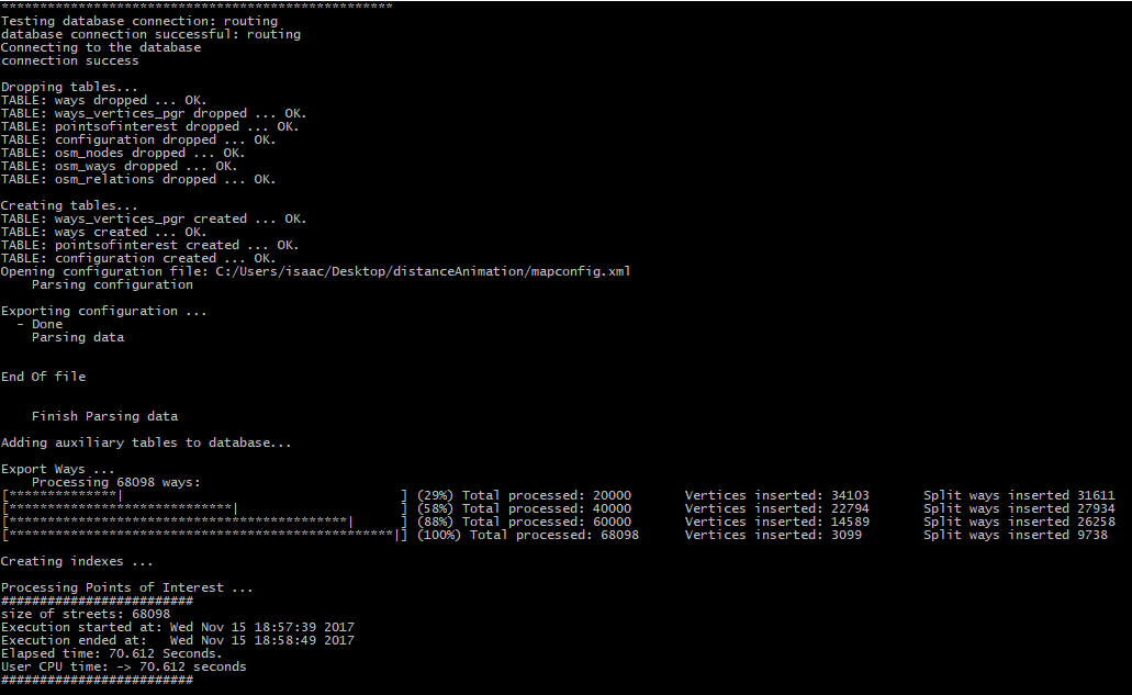
Step 4: Creating the database view
Open pgAdmin, create a new script (in pgAdmin 4 do a right click in the routing database and select CREATE script) and run the following queries:
- Enable the pgrouting extension on the database
CREATE EXTENSION pgRouting;
- We need to select the node where the animation starts. To do it we can compute the centroid of all the Point set so it starts from the center and get the nearest node to that point or get the nearest node to a pair of coordinates. In any case, write down the starting node id as we will need it later.
- Getting the center node
SELECT id
FROM ways_vertices_pgr
ORDER BY CAST (st_DistanceSphere(the_geom, (SELECT ST_AsText(st_centroid(st_union(the_geom)))
FROM ways_vertices_pgr)) AS INT) ASC
LIMIT 1;
- Getting the nearest node to a pair of coordinates
SELECT id
FROM ways_vertices_pgr
ORDER BY CAST (st_DistanceSphere(the_geom, st_setsrid(st_makepoint(longitude, latitude), 4326)) AS INT) ASC
LIMIT 1;
- Getting the center node
- Compute the distance from a given node to all of them.
The query has two parameters: the starting node id you have written down before and the maximum cost of the traversal in seconds. You should run the following query until the agg_cost of the first row is less than the maximum cost you have specified. Write down the agg_cost of the first row as we’ll need it in the next steps.SELECT seq, node, edge, distances.cost, agg_cost, edges.the_geom FROM pgr_drivingDistance( 'SELECT osm_id AS id, source, target, cost_s AS cost, reverse_cost_s AS reverse_cost FROM ways', 1, -- this is the starting node id (the one you wrote down before!) 50000 -- this is the maximum cost (seconds in this case) ) AS distances LEFT JOIN ways edges ON edges.osm_id=distances.edge ORDER BY agg_cost DESC; - Create a view to use with QGIS with the following query. You should change the node id parameter to the one you used in the previous query and the maximum cost to the value you wrote down in the previous step.
CREATE OR REPLACE VIEW edges_1_10343 AS
SELECT row_number() OVER (), edge, node, distances.cost, agg_cost, edges.the_geom FROM pgr_drivingDistance(
  'SELECT osm_id AS id, source, target, cost_s AS cost, reverse_cost_s AS reverse_cost
    FROM ways',
    1,  -- this is the start node id (the same as the previous query!)
    10343     -- this is the maximum cost (the agg_cost column value of the first row of the previous query)
  ) AS distances
  LEFT JOIN ways edges ON edges.osm_id=distances.edge;
Step 5: Getting the data into QGIS
Open QGIS and create a new connection with our database.
- Go to Layer -> Add layer -> Add PostGIS layer
- Press New under the Connections group. A panel will open where you’ll need to write the connection parameters of the database. In our case set the server field as localhost, routing as the database and the username and password used when the database was installed. Name the connection and press Ok. If everything has gone well you should see the connection in the Connections group.
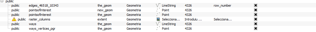
- Select your just created connection from the dropdown and press Connect. A list of all the possible layers to import will be shown. You will see a row called edges_1_10343 with a warning sign before public. The warning is shown because QGIS can’t detect a primary key. What we’ll need to do is select row_number in the object id dropdown and then select it and press Add
Step 6: Styling the data and creating the video
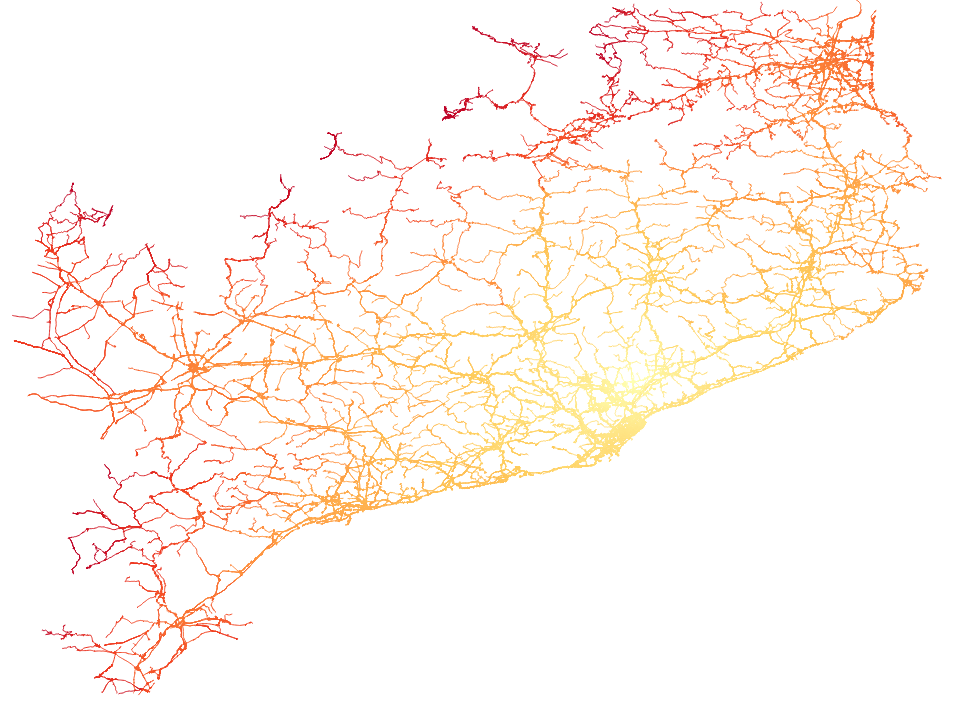
What we’ll do is create a linear color ramp that maps the agg_cost of each edge to a [0, 1] inteval where a cost of 0 is mapped to the starting color of the ramp and the maximum agg_cost value is mapped to the ending color of the ramp.
- Right click on the edges_1_10343 layer and select Properties
- Under the Style tab, select simple line, press the data driven property icon
 next to the color attribute and select edit. That will open a window to build expressions. Copy the following expression on it, change the maximum_value to the one you wrote down when you ran the queries and press Ok twice.
ramp_color( 'YlOrRd', scale_linear( "agg_cost", 0, maximum_value, 0, 1))
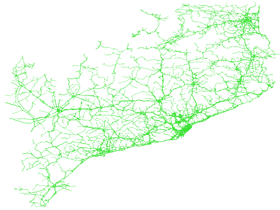
You will get something like this with your geometry
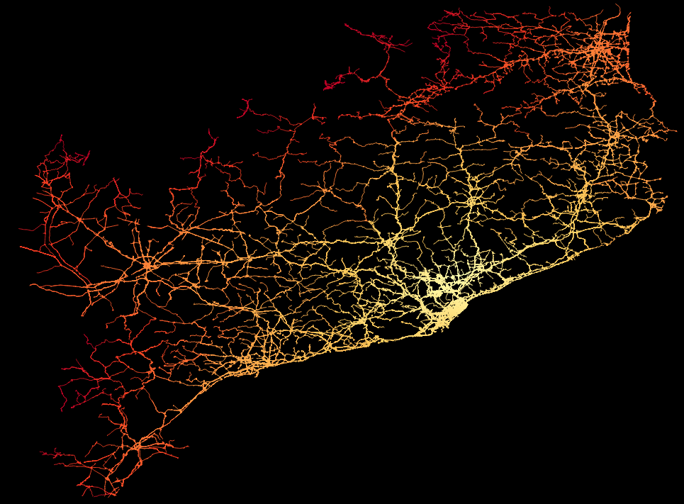
- Change the background color to black by going to Project -> Project properties. In the General tab press the selector next to the background color and select the black one.
- Press the Settings button in the Time Manager panel to configure the animation
- Press Add layer, select your layer, set agg_cost as the start time, No end time – accumulate features as the End time and press Ok
- Under Animation Options set the Show frame for value to 16 milliseconds to do a 60fps video
- Disable the Display frame start time on map checkbox if you don’t want the time to be shown and press Ok. If everything has gone well, the map panel should now show just the start of the animation.

- Now we need to compute what each animation step amounts to. If we want want to generate a 4 seconds video we must divide the maximum agg_cost value you wrote down before by 60*4 and set the Time frame size value and the dropdown next to it acoordingly. For example, if we have a maximum agg_cost of 10343 seconds we should set the animation step to 10343/(60*4) = 43 seconds.
- Press the Export Video button in the Time Manager panel, select an output folder, select Frames Only as the output and press Ok. The Time Manager plugin will now start to render each video frame and save it as a png file in the output folder you specified.
- We should now have a folder full of png files with each one being a frame of our video. To generate an mp4 video from those png we’ll use the following command from the root of the folder where you installed ffmpeg
./ffmpeg -framerate 60 -i /path/To/frame%04d.png -vcodec libx264 -preset slow -b:v 4096k ./output.mp4
After the process finishes now you should have your own Time-to animation video.
Here you have some more examples:
Lyon
Rome
Tokyo
Giving credit where its due
- Inspiration came from this article. I’ve expanded and updated some bits of it to make a step-by-step guide out of it.
- The dark background in the videos is a customized Mapbox Dark theme where the labels are removed
Hope you gals and guys have enjoyed this step by step guide!